“Whenever you find yourself on the side of the majority, it is time to pause and reflect.” [Mark Twain]

Abstract

SUMPRODUCT is a very powerful function. You can conditionally count or sum large ranges of data. On the other hand, if you need to maintain statistics on all elements of a larger list, the manual maintenance effort and sometimes the runtime of a recalculation can be too high.

Advantages of using SUMPRODUCT: SUMPRODUCT is more flexible than COUNTIF or SUMIF which support ONE condition only.

Example 1

If you want to count all cells in A1:A100 which show a positive numerical value, e.g. which are greater zero:

=COUNTIF(A1:A100,">0")

can be replaced by

=SUMPRODUCT(--(A1:A100>0))

And if you need to count how many numbers of A1:A100 are greater than zero AND where the string in column B is “LONDON”, use

=SUMPRODUCT(--(A1:A100>0),--(B1:B100="LONDON"))

This cannot be done with COUNTIF. Instead of using SUMIF if you can sum up conditionally with SUMPRODUCT.

Example 2

If you want to sum up all cells in B1:B100 where the corresponding cells in A1:A100 show a positive numerical value:

=SUMIF(A1:A100,">0",B1:B100)

can be replaced by

=SUMPRODUCT(--(A1:A100>0),B1:B100)

Please note that the double unary minus translates the Boolean values True and False into the numbers 1 and 0. You could also have used 0+ or 1* to do this but I think the double unary minus canonically indicates a condition and if that’s missing you know that you look at the values which you need to sum up. Now the fun starts because you can combine conditions which COUNTIF and SUMIF cannot deal with - since there are more than one of them.

Example 3

[AND Condition] If you want to add all numbers in C1:C100 where A1:A100 are negative and where B1:B100 show a YES:

=SUMPRODUCT(--(A1:A100<0),--(B1:B100="YES"),C1:C100)

[OR Condition] If you want to add all numbers in C1:C100 where A1:A100 are negative or where B1:B100 show a YES:

=SUMPRODUCT(SIGN((A1:A100<0)+(B1:B100="YES")),C1:C100)

Note: The SIGN function reduces possible overlapping OR criteria - which would sum up to more than one - to one exactly! I suggest to always wrap OR criteria checks into a SIGN() function. A simple sum is naive and outright dangerous because a less skilled person could amend non-overlapping XOR criteria to overlapping OR ones.

More Complex Examples

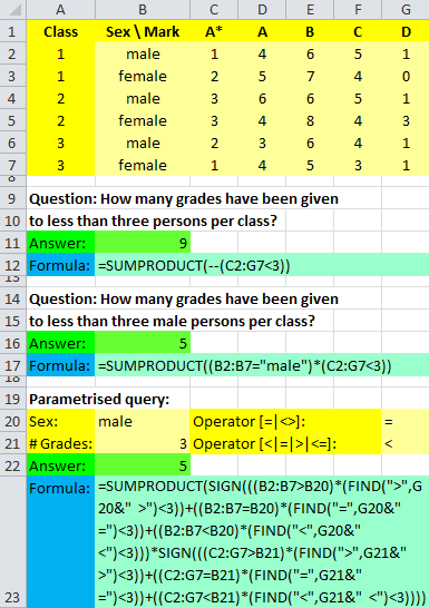
Please note that I normally prefer SUMPRODUCT(–(),–()) to SUMPRODUCT(()())* because this separates the conditions quite clearly, but for multi-column ranges such as in cell B17 above you can only use the *-approach.

SUMPRODUCT offers you a nice and complex functionality of an array function. You can count and sum up attributes/properties of cell ranges and put the result into a cell. If you need to do this for all appearing characteristics you face some difficulties, though. You need to prepare the set of unique characteristics for use with SUMPRODUCT first. If you do this manually you end up with manual maintenance if your input changes. If you want to do this with worksheet functions you increase the complexity of your worksheet.

Yet Another Example

If you need to count all different strings in a column and to list them together with their number of occurrences, for example, you have two reasonable options for a worksheet function approach with SUMPRODUCT:

a) To manually write down all different entries and to count these with COUNTIF or SUMPRODUCT. You would have to maintain this list manually then.

b) A feed of unique values with worksheet functions increases the complexity of the worksheet (please see here).

For cases like this I suggest to use a Pivot table or to use my user-defined-function (UDF) sbMiniPivot instead of SUMPRODUCT or COUNTIF.

Also, if you want to sum up specified cells for all occurring corresponding cells/combinations, use a Pivot table or again sbMiniPivot, please.

A Comparison of Three Different Approaches

A comparison of three different approaches to form a statistic on about 30,000 records of data:

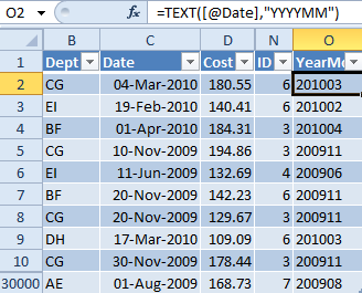
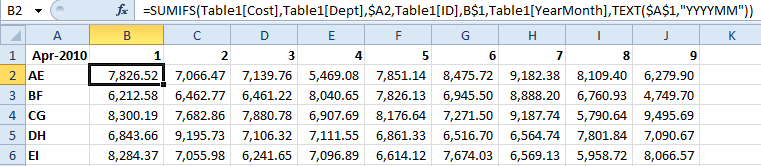
We have a data table with 30,000 rows of data: Each row consists of a department key, a date, cost and identifier. Now we want to show for April 2010 the accumulated costs per department (leftmost column) and per identifier (topmost row).

Worksheet Formulas

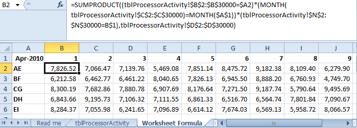
Sheet “Worksheet Formula” is built with SUMPRODUCT worksheet formulas. You need to specify all different departments and Id’s correctly and completely or the statistic will not be correct. The MONTH-part of the formula is dangerous because data might be older than 1 year. This sheet needs about 1,200ms (1.2s) to be calculated (please see sheet “FastExcel” for details).

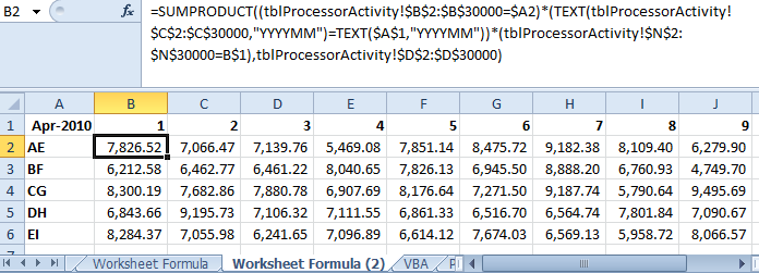
Sheet “Worksheet Formula (2)” is also built with SUMPRODUCT worksheet formulas. It fixes the MONTH issue but its runtime is about 10,600ms (10.6s).

Sheet “Worksheet Formula (3)” is built with SUMIFS worksheet formulas. It needs a helper column YearMonth in sheet tblProcessorActivity and runs about 270ms + 110ms = 0.38s.

VBA

Sheet “VBA” is built with a VBA macro. All different departments and Id’s will be collected automatically. This sheet needs about 860ms (0.86s) to be calculated (according to FastExcel). Please note that this code also uses the class SystemState.

Please read my Disclaimer.

Option Explicit

'Enumerate source sheet columns - easier to maintain later
Enum tblProcessorActivity_Columns
    tpa_Department = 2
    tpa_Date
    tpa_Cost
    tpa_Id = 14
End Enum 'tblProcessorActivity_Columns

Const CSep = ","

Sub CurrentMonthsCost()
'Source (EN): http://www.sulprobil.de/sumproduct_en/
'Source (DE): http://www.berndplumhoff.de/summenprodukt_de/
'(C) (P) by Bernd Plumhoff 20-Jan-2013 PB V0.11
Dim objCosts As Object, objDepts As Object, objIds As Object
Dim lRow As Long, lDeptCount As Long, lIdCount As Long
Dim dtMaxDate As Date
Dim sMaxDateYYYYMM As String, sIdx As String
Dim v As Variant, vDeptId As Variant
Dim state As SystemState
Set state = New SystemState

Set objCosts = CreateObject("Scripting.Dictionary")
Set objDepts = CreateObject("Scripting.Dictionary")
Set objIds = CreateObject("Scripting.Dictionary")
Sheets("VBA").Select
Cells.ClearContents
With Sheets("tblProcessorActivity")
dtMaxDate = Application.WorksheetFunction.Max(.Range("C2:C30000"))
sMaxDateYYYYMM = Format(dtMaxDate, "YYYYMM")

'Main data processing loop
lRow = 2
Do While Not IsEmpty(.Cells(lRow, tpa_Department))
    If sMaxDateYYYYMM = Format(.Cells(lRow, tpa_Date), "YYYYMM") Then
        sIdx = .Cells(lRow, tpa_Department) & CSep & .Cells(lRow, tpa_Id)
        objCosts.Item(sIdx) = objCosts.Item(sIdx) + .Cells(lRow, tpa_Cost)
    End If
    lRow = lRow + 1
Loop

'We are almost finished - rest is formatting output
Cells(1, 1) = dtMaxDate
For Each v In objCosts.keys
    vDeptId = Split(v, CSep)
    If objDepts.Item(vDeptId(0)) = 0 Then
        lDeptCount = lDeptCount + 1
        objDepts.Item(vDeptId(0)) = lDeptCount
        Cells(lDeptCount + 1, 1) = vDeptId(0)
    End If
    If objIds.Item(vDeptId(1)) = 0 Then
        lIdCount = lIdCount + 1
        objIds.Item(vDeptId(1)) = lIdCount
        Cells(1, lIdCount + 1) = vDeptId(1)
    End If
    Cells(objDepts.Item(vDeptId(0)) + 1, objIds.Item(vDeptId(1)) + 1) = _
        objCosts.Item(v)
Next v
End With

'Sort result row-wise by department and column-wise by Id
'Surely you could and you maybe even would prefer Excel's built-in sort ...
'Please include code from http://sulprobil.de/html/gsort.html
Range(Cells(2, 1), Cells(lDeptCount + 1, lIdCount + 1)).FormulaArray = _
    GSort(Range(Cells(2, 1), Cells(lDeptCount + 1, lIdCount + 1)))
Range(Cells(1, 2), Cells(lDeptCount + 1, lIdCount + 1)).FormulaArray = _
    Application.WorksheetFunction.Transpose(GSort( _
    Application.WorksheetFunction.Transpose(Range(Cells(1, 2), _
    Cells(lDeptCount + 1, lIdCount + 1))), "A", "N"))

End Sub

Pivot Table

Sheet “Pivot” is showing a pivot table. All different departments and Id’s will be collected automatically. But you need to filter the date range manually. It is being refreshed by a VBA macro. This sheet needs about 170ms (0.17s) to be refreshed (according to FastExcel) plus your manual time to filter the date range.

Option Explicit

Sub RefreshPivotTable()
ActiveSheet.PivotTables("PivotTable1").PivotCache.Refresh
End Sub

Runtimes have been calculated on my dual core laptop.

Please read my Disclaimer.

sbSumproductComparison.xlsm [1744 KB Excel file, open and use at your own risk]